Matrix Factorization in Recommender System
Abstract: Recommender system is still a hot research topic in computing math and computer science. In 2006, Netflix held a competition called Netflix Prize to find an efficient recommender system algorithm. Although deep learning works well in recommender system, it is still important to learn and improve traditional algorithms including collaborative filtering and matrix factorization. In fact, those traditional algorithms are still widely used. In this paper, we introduced the basic notion of matrix factorization and discussed some classic algorithms. We also proposed an improved algorithm based on bias SVD. Finally, we tested these algorithms on a dataset, and compared their accuracy.
Intruduction
With the rapid development of computer science and internet economy, many researchers are focusing on recommender system. Recommender system plays an important role indot-com companies, such as Amazon, Google and Netflix. The main purpose of recommender system is connecting users and information. On one hand, users can easily find useful information. On the other hand,providers can push information to users point-to-point. Generally, recommender system is similar to rate prediction. In other words, we need to predict users' future rates based on their profiles and the properties of items.
Recommender system was proposed in 1992 for the first time. With the efforts of researchers, now recommender systems have various algorithms such as Collaborative Filtering, Frequent Itemset, Cluster Analysis, Regression analysis,Graphical Model, Restricted Boltzmann Machine, Tensor Decomposition, and Deep Learning.
However, researchers are still facing data sparsity problem. If we treat the data as a matrix, then the dimension is extremely large, while only some of the entries have nonzero values. Large dimension means that we can not store theentire matrix and the time complexity should be less enough. Usually, the dimension of data matrix is up to $10^5$. In this case, even $O(n^2)$ time complexity is unacceptable. Therefore, we have to use dimensionality reduction to solve it.
We will introduce matrix factorization to reduce the dimension and establish the recommender system. The rest of this paper is structured as follows. Section 2 introduces the matrix factorization in recommender system. Section 3 introduces sometraditional algorithms. In section 4, we propose an improved algorithm. In section 5, we apply those algorithms to a real problem.Finally, Section 6 concludes.
Matrix Factorization
Consider a recommender system: there are m users and n items, and each user have rated some (a few) items. Now we collect those data together and denote by a matrix, says $M$. Since it is sparse, the matrix should look like:
\[ M=\begin{pmatrix} 1,0,0,0,2 \\ 0,0,3,0,0 \\ 0,0,0,0,0 \\ 0,0,0,0,0 \\ 0,4,0,0,0 \end{pmatrix}\]
Since the dimension of $M$ can be extremely large, traditional singular value decomposition (SVD) may not work. One of the solutions is using truncated SVD, only picking the first $k$ largest singular values and their corresponding eigenvectors.Another one is Funk-SVD, which was proposed by Simon Funk in 2006. Instead of decompose $M$ into three matrices, we only need to find two matrices $P$ and $Q$ s.t.
\[ M=PQ \]
where $P$ is m-by-k and $Q$ is k-by-n. Since we can let $k$ small enough, $M$ can be stored in form of $P,Q$. For example, suppose int takes 4 bytes, then a $105$-by-$105$ matrix will occupy approximately 37G memory, while two $105$-by-$102$ matrices only occupy 72M memory, which is acceptable even on personal computer.If we successfully decompose $M$ into $P,Q$, we can compute the (U,I)'th entries of $M$ by $P$ and $Q$, which means that we can predict the score of item I rated by user U. Hence, $P$ contains all the properties of users and $Q$ contains all the properties of items. We will call $P$ user matrix and $Q$ item matrix.For example, consider the matrix $M$:
\[ M=\begin{pmatrix} 1,0,0,0,2 \\ 0,0,3,0,0 \\ 0,0,0,0,0 \\ 0,0,0,0,0 \\ 0,4,0,0,0 \end{pmatrix}\]
Suppose it has a Funk-SVD:
\[ P=\begin{pmatrix} P_1 \\ P_2 \\ P_3 \\ P_4 \\ P_5 \\ \end{pmatrix} Q=\begin{pmatrix} Q_1,Q_2,Q_3,Q_4,Q_5 \end{pmatrix}\]
Then, the score of an item, says $I=4$, rated by a user, says $U=1$, is exactly the value of $P_1Q_4$.Now our goal is to find such two matrices. Although $M$ can not be decomposed directly, we still can use iteration method to build the decomposition. Suppose we have matrices $P,Q$, then we can write
\[ M'=PQ \]
and its (U,I)'th entries is:
\[ M_{UI}'=\sum_{k} P_{Uk}Q_{kI} \]
We want the error between $M$ and $M'$ as small as we can. Consider sum of square error (SSE):
\[ SSE=\sum_{(U,I)\in S_M}(M_{UI}-M'_{UI})^2 \]
and root mean square error (RMSE)
\[ RMSE=\sqrt{\frac{SSE}{N}} \]
where $S_M={(a,b)\ :\ M_{ab}\neq 0}$, i.e. $S_M$ contains the positions of all the nonzeros in $M$.Therefore, the original problem becomes:
\[ argmin_{P,Q} \sqrt{\frac{\sum_{U,I}(M_{UI}-\sum_{k}P_{Uk}Q_{kI})^2}{N}} \]
which is exactly an optimization problem.
Traditional Algorithms
Funk-SVD
As we discussed above, Funk-SVD requires solving an optimization problem
\[ argmin_{P,Q} \sqrt{\frac{\sum_{U,I}(M_{UI}-\sum_{k}P_{Uk}Q_{kI})^2}{N}} \]
We can use gradient descent to solve this. Consider the objective function
\[ RMSE=\sqrt{\frac{\sum_{U,I}(M_{UI}-\sum_{k}P_{Uk}Q_{kI})^2}{N}} \]
which is a function of $P$ and $U$. Fix $U,I$, then we can compute the partial derivative of $RMSE$:
\[ \frac{\partial}{\partial P_{Uk}} RMSE=-\frac{1}{RMSE}\left( M_{UI}-\sum_{k} P_{Uk}Q_{kI} \right)Q_{kI} \]
\[ \frac{\partial}{\partial Q_{kI}} RMSE=-\frac{1}{RMSE}\left( M_{UI}-\sum_{k} P_{Uk}Q_{kI} \right)P_{Uk} \]
Hence, at each step, we can update $P,Q$ by
\[ P_{Uk}=P_{Uk}+\alpha\frac{1}{RMSE}\left( M_{UI}-\sum_{k} P_{Uk}Q_{kI} \right)Q_{kI} \]
\[ Q_{kI}=Q_{kI}+\alpha\frac{1}{RMSE}\left( M_{UI}-\sum_{k} P_{Uk}Q_{kI} \right)P_{Uk} \]
where $\alpha$ is a parameter.
Now let's check whether this algorithm works. Consider the same matrix
\[ M=\begin{pmatrix} 1,0,0,0,2 \\ 0,0,3,0,0 \\ 0,0,0,0,0 \\ 0,0,0,0,0 \\ 0,4,0,0,0 \end{pmatrix}\]
By using Funk-SVD, we can get two matrices $P,Q$:
\[ P=\begin{pmatrix} 1.1012 & 0.7452 & 0.9319 \\ 1.0791 & 0.7190 & 1.2594 \\ 0. & 0. & 0. \\ 0. & 0. & 0. \\ 0.9866 & 1.2673 & 1.0993 \\ \end{pmatrix}\]
\[ Q=\begin{pmatrix} 0.1335 & 1.2925 & 0.7550 & 0. & 0.6452 & \\ 0.1752 & 1.4527 & 0.5107 & 0. & 0.4116 & \\ 0.7750 & 0.7277 & 1.4434 & 0. & 1.0544 & \\ \end{pmatrix}\]
and
\[ M'=\begin{pmatrix} 1. & 3.1843 & 2.5572 & 0. & 2. \\ 1.2463 & 3.3560 & 3. & 0. & 2.3203 \\ 0. & 0. & 0. & 0. & 0. \\ 0. & 0. & 0. & 0. & 0. \\ 1.2059 & 3.9165 & 2.9791 & 0. & 2.3175 \\ \end{pmatrix}\]
Comparing $M'$ with $M$, we can see that for $(U,I)\in S_M$, $M_{UI}\approx M'_{UI}$, and some blanks in $M$ have been filled with proper values.
Regularized SVD
In order to avoid overfitting, we can add regularization parts in Funk-SVD. In this case, we have
\[ \begin{aligned} SSE = & \sum_{(U,I)\in S_M}(M_{UI}-M'_{UI})^2 \\ & +\lambda\left(\sum_U|P_U|_2^2 +\sum_I|Q_I|_2^2 \right) \end{aligned}\]
where $P_U$ is the $U$'th row vector of $P$ and $Q_I$ is the $I$'th column vector of $Q$; $\lambda$ isthe regularization parameter.Consider the derivative of $|P_U|_2^2$. Since $\frac{\partial}{\partial x}(xTAx)=(A+AT)x$, we have
\[ \begin{aligned} \frac{\partial}{\partial P_U}|P_U|_2^2 & =\frac{\partial}{\partial P_U}\left(P_U^T P_U\right) \\ & =2P_U \end{aligned}\]
Therefore, the updating formulas become:
\[ \begin{aligned} P_{Uk}= & P_{Uk}+\alpha\frac{1}{RMSE}\left( M_{UI}-\sum_{k} P_{Uk}Q_{kI} \right)Q_{kI} \\ & -\alpha\frac{1}{RMSE}\lambda P_{Uk} \end{aligned}\]
\[ \begin{aligned} Q_{kI}= & Q_{kI}+\alpha\frac{1}{RMSE}\left( M_{UI}-\sum_{k} P_{Uk}Q_{kI} \right)P_{Uk} \\ & -\alpha\frac{1}{RMSE}\lambda Q_{kI} \end{aligned}\]
Bias SVD
It may be insufficient to only consider the connection between users and items. In fact, different users have different evaluation criterions. Someusers may prefer to give low scores (less than average) to every item, or give high scores (like 5-stars) regardless of the quality of the items. Similarly,some items may have perfect quality so that most users gave good rates, or the quality is disappointed so that most users gave bad rates. Hence, we have toadd the properties of both users and items to our algorithm.
Suppose the average of $M$ is $\sigma$. For $U$'th user, we call this user's preference a \textbf{bias}, denoted by $b_U$, which is a real number (can be negative). Similarly, for $I$'th item,we have $b_I$.In this case, the decomposition becomes:
\[ M_{UI}'=\sigma+b_U+b_I+\sum_k P_{Uk}Q_{kI} \]
and the error function becomes:
\[ \begin{aligned} SSE = & \sum_{(U,I)\in S_M}(M_{UI}-M'_{UI})^2 \\ & +\lambda\Big(\sum_U|P_U|_2^2 +\sum_I|Q_I|_2^2 \\ & + \sum_U|b_U|2+\sum_I|b_I|2 \Big) \end{aligned}\]
Additionally, we have to update $b_U$ and $b_I$ at each step. Hence, the updating formulas are:
\[ \begin{aligned} P_{Uk}= & P_{Uk}+\alpha\frac{1}{RMSE}\left( M_{UI}-\sum_{k} P_{Uk}Q_{kI} \right)Q_{kI} \\ & -\alpha\frac{1}{RMSE}\lambda P_{Uk} \end{aligned}\]
\[ \begin{aligned} Q_{kI}= & Q_{kI}+\alpha\frac{1}{RMSE}\left( M_{UI}-\sum_{k} P_{Uk}Q_{kI} \right)P_{Uk} \\ & +\alpha\frac{1}{RMSE}\lambda Q_{kI} \end{aligned}\]
\[ \begin{aligned} b_U= & b_U+\alpha \frac{1}{RMSE}\Big( M_{UI}-M'_{UI} \\ & -\lambda b_U \Big) \end{aligned}\]
\[ \begin{aligned} b_I= & b_I+\alpha \frac{1}{RMSE}\Big( M_{UI}-M'_{UI} \\ & -\lambda b_I \Big) \end{aligned}\]
SVD++
In reality, users may view a item without rating. In fact, we can suppose these users were interested in this item, since they may be attracted by the description such as pictures and titles.
We call these information implicit feedback. Since the rating matrix is sparse, we need implicit feedback to improve our algorithms. Generally, implicit feedback are greatly larger thanrating records.
We denote all the items that the $U$'th user provided implicit feedback by $F(U)$. Then the decomposition becomes:
\[ \begin{aligned} M_{UI}'= & \sigma+b_U+b_I+\sum_k P_{Uk}\cdot \\ & \left(Q_{kI}+|F(U)|^{-1/2}\sum_{j\in F(U)}y_{jk}\right) \end{aligned}\]
and the error function becomes:
\[ \begin{aligned} SSE = & \sum_{(U,I)\in S_M}(M_{UI}-M_{UI}')^2 \\ & +\lambda\Big(\sum_U|P_U|^2_2 +\sum_I|Q_I|^2_2 \\ & + \sum_U|b_U|2+\sum_I|b_I|2 \\ & +\sum_{j}|y_j|^2_2 \Big)
\end{aligned} \]
Note that $y_j$ are variables that need to be updated. Their updating formulas are:
\[ \begin{aligned} y_j= & y_j+\alpha \frac{1}{RMSE}\Big( M_{UI}-M'_{UI}\Big)|F(U)|^{-1/2} \\ & -\alpha \frac{1}{RMSE}\lambda\ y_j \end{aligned}\]
Bias SVD with weight
Now we propose an improved algorithm. We noticed that some users had rated many items, while some users had only rated a few items (even 1 or 2 item(s)).
It is clear that if a user rated a large number of items, its contribution to the recommender system should be greatly useful.Based on this, we added weight to each user, denoted by $\omega_U$, which is related to the number of items rated by $U$'th user. In this case, when we update $Q_I$, the updating formula becomes:
\[ \begin{aligned} Q_{kI}= & Q_{kI}+\alpha\frac{1}{RMSE}\left( M_{UI}-\sum_{k} P_{Uk}Q_{kI} \right)\omega_U P_{Uk} \\ & +\alpha\frac{1}{RMSE}\lambda Q_{kI} \end{aligned}\]
Application and Comparison
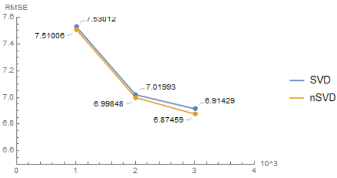
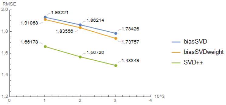
In this section, we will use Book-Crossing Dataset to test our algorithms and compare their accuracy.This dataset has up to $10^5$ users' rating records among $10^5$ different books. Also, this dataset provides implicit data. Due to the limitation of laptop's CPU, we only test $10^3,2\cdot 10^3,3\cdot 10^3$ many data.Codes are available on GitHub


We can see that with the consideration of bias, the accuracy rapidly increased, from about $7.0$ to $1.8$. With the consideration of weights, the accuracy increased a little, compared with biasSVD. Furthermore, SVD++ have the most accuracy among algorithms we discussed before.
Conclusion
Matrix factorization provides a efficient method for us to establish the recommender system. Since we do not need to store the entire rating matrix, the algorithms can be run even on personal computer with limited performance. However, the speed of algorithms becomes significantly slow when the dimensions increase. One of the solution is change gradient descent to stochastic gradient descent, which generally performs faster.
However, matrix factorization still has its disadvantage. If our rating matrix changes, for example, we add some new users and their rating records, then we have to run the whole algorithm again, even though the changes are slight. In fact, the rating record is dynamic in reality, and it is inefficient to update the recommender system in this way. Fortunately, we can combine traditional algorithms with deep learning, which allow us to update our system online.
References
- Improving Recommendation Lists Through Topic Diversification, Cai-Nicolas Ziegler, Sean M. McNee, Joseph A. Konstan, Georg Lausen; Proceedings of the 14th International World Wide Web Conference (WWW '05), May 10-14, 2005, Chiba, Japan.
- Koren Y, Bell R, Volinsky C. Matrix factorization techniques for recommender systems[J]. Computer, 2009 (8): 30-37]
- Salakhutdinov R, Mnih A. Probabilistic matrix factorization. NIPS, 2008.
- Rendle, Steffen. "Factorization machines." Data Mining (ICDM), 2010 IEEE 10th International Conference on. IEEE, 2010.
